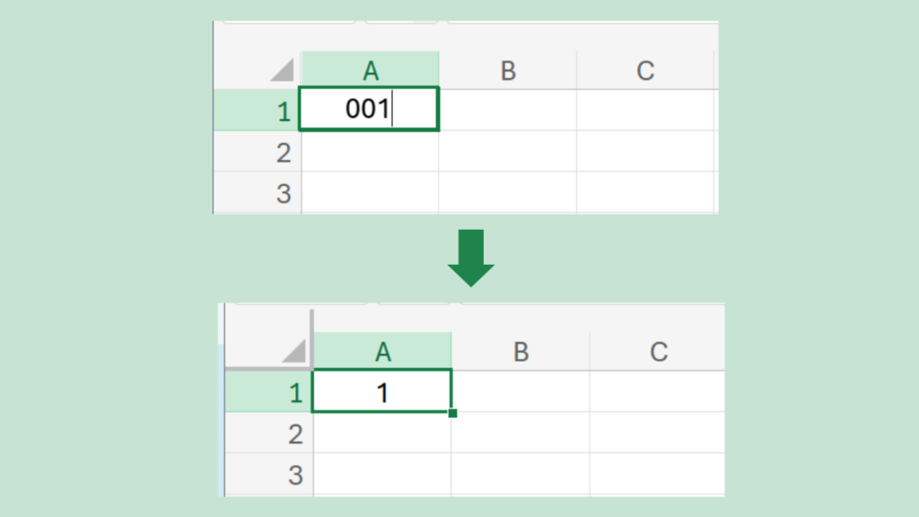
When you try to input “001” in Excel, it often displays as “1.” This happens because Excel automatically interprets “001” as a number, and leading zeros are removed. Here are three simple methods to display “001” instead of “1” in Excel.

1. Add an Apostrophe at the Beginning
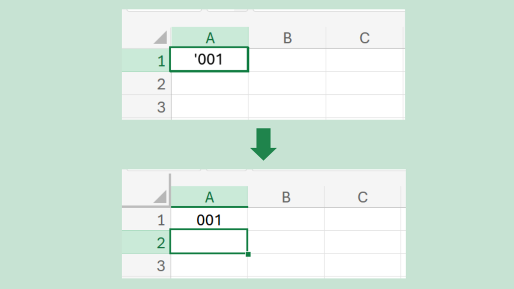
To display a number with leading zeros, you can add an apostrophe (‘) at the beginning of the input.

Example:
- Input: ‘001
- Result: The cell displays “001”
2. Format the Cell as Text
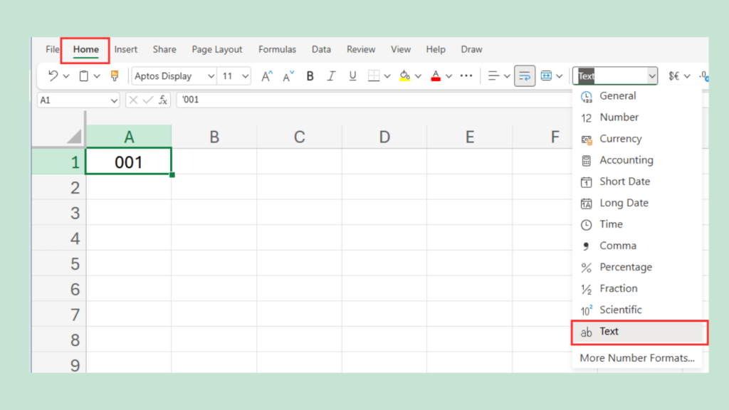
You can also format the cell as text before entering the number. This ensures that Excel treats the input as text and preserves any leading zeros.

Steps
- Select the target cell(s).
- Go to the Home tab.
- In the Number section, select Text from the dropdown menu.
- Enter “001” into the cell.
- The cell will display “001” as entered, without removing the leading zeros.0
3. Use Custom Number Formatting
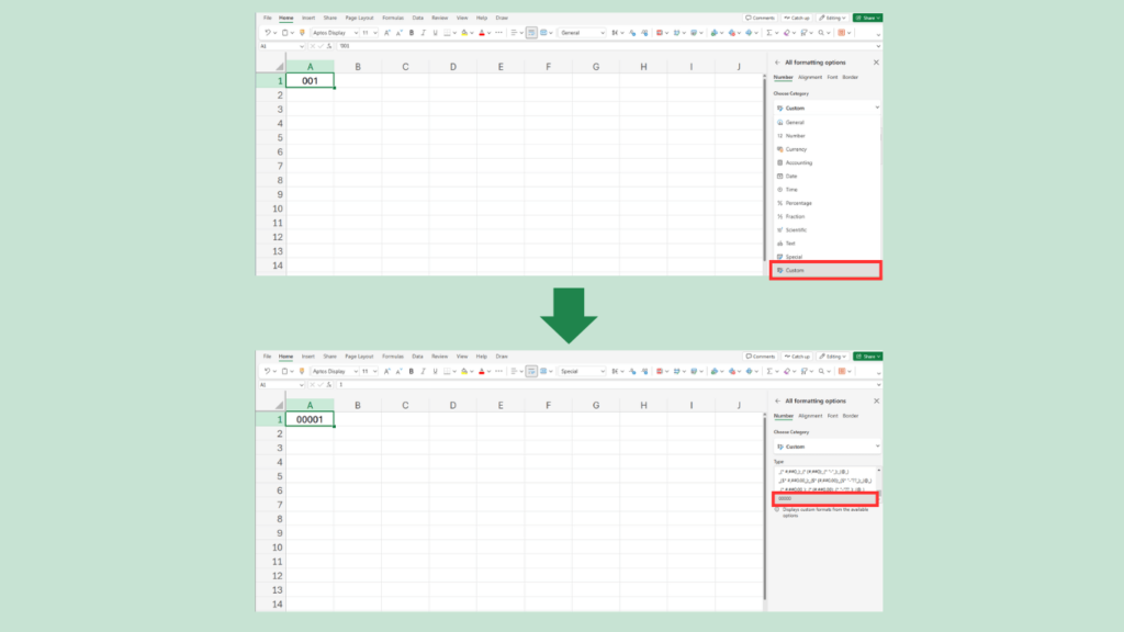
For numerical data, you can use custom formatting to display leading zeros.

Steps:
- Select the target cell(s)
- Press Ctrl + 1 to open the Format Cells dialog box (Note: Do not use the numeric keypad for this shortcut)
- Choose Custom from the Category list
- In the Type field, enter 00000
Now, when you enter “1,” it will display as “00001.”
Note: If you input “10,” it will display as “010.”
Summary
These are the three methods to display leading zeros in Excel:
1. Add an Apostrophe: Treats the input as text and preserves the zeros.
2. Format as Text: Ensures the cell always treats input as a text string.
3. Custom Formatting: Displays numbers with leading zeros while keeping them as numeric data.
Try these methods to keep your data in the desired format!
